Sparse modeling

1. A Sparse PCA for Nonlinear Fault Diagnosis and Robust Feature Discovery of Industrial Processes

Introduction

Modern industrial processes comprise of a large number of nonlinear subsystems. These subsystems also interact with each other in a complex fashion. In most cases, it is difficult to obtain an explicit model to accurately describe the dynamical behavior of the systems.

It is noticed that the main source of the weaknesses of the standard PCA model is the use of Pearson’s dependence measure. An outlier data sample deviating considerably from the mean (center) of the data distribution causes signiﬁcant distortion of the covariance matrix. This distortion may induce the extraction of unnecessary eigenvectors in the direction of outlier data samples to account for the additional variance.

Methods

Industrial process data samples are robustly standardized using their median and median absolute deviation (MAD).
the Spearman’s and Kendall tau’s rank correlation coefﬁcients are computed for each pair of process variables to form the rank correlation matrix. The Spearman’s and Kendall tau’s rank correlation coefﬁcients are robust to outliers.
a set of eigenvectors retaining the nonlinear correlation structures of the process data are extracted from the rank correlation matrix to construct the feature space.
a generalized iterative deﬂation procedure22 is applied to the rank correlation matrix to extract sparse eigenvectors.

Cases

No not really complex system. A simple real case and the TE process.

2. Improved fault detection and diagnosis using sparse global-local preserving projections

#sparse-modeling

Introduction

A common drawback of dimensionality reduction methods is the lack of sparsity in their solutions. A common drawback of dimensionality reduction methods is the** lack of sparsity in their solutions**. The sparse representation of PCA has been widely investigated.

Although sparse PCA (SPCA) has better interpretability than PCA, it inherits a disadvantage from PCA. This disadvantage is that both SPCA and PCA only preserve the global Euclidean structure (i.e., data variance) of data but totally neglect the local data structure (i.e., local neighborhood relations among data points). Because the local neighborhood structure is also a very important aspect of data features, neglecting such important data information inevitably degrades the performance of PCA and SPCA. Consequently, PCA and SPCA cannot fully extract useful information from data. Moreover, PCA and SPCA are easier to be affected by outliers and noises.

A monitoring model without sparsity has three drawbacks in fault detection and fault diagnosis.

First, it fails to** reveal meaningful process mechanisms** and control loops between process variables from process data. This drawback hinders the analysis and interpretation of monitoring results.

Second, because of the lack of sparsity, a monitoring model may suffer from the redundant coupling and interferences between process variables, which reduces the fault sensitivity and the fault detection capability.

Third, based on a monitoring model without sparsity, it is hard to accurately evaluate the effect of faults on each process variable, which may reduce the reliability and accuracy of fault diagnosis.
In real industrial processes, there are complicated coupling between process variables, and thus faults may propagate between different process variables. In addition, a fault may do more harm to other process variables rather than the variables that cause the fault.

Methods

Use Sparse Global-local preserving projections method to preserve both global and local structure of data.

Cases

TE process

3. A Sparse Reconstruction Strategy for Online Fault Diagnosis in Nonstationary Processes with No a Priori Fault Information

#sparse-modeling #nonstationary

Introduction

Fault detection and diagnosis for nonstationary process monitoring is a difficult task because the fault signal may be buried by non- stationary trends resulting in a low fault detection rate. The time series $x_{t}$ is said to be weakly stationary if it shows a time-varying mean or a time-varying variance or both.

Although the data-differencing process can turn the nonstationary time series into a stationary one, this preprocessing can cause loss of dynamic information and fault features in the data that lead to poor fault detection and diagnosis performance. It is very difficult to isolate the faulty variables for the nonstationary processes since the abnormal signals may not be clearly distinguished from normal nonstationary trend whose statistical characteristics are changing with time.
the nonstationary variables in the nonstationary processes correlate to each other, and those nonstationary variables maintain a long-run dynamic equilibrium relation governed by the physical mechanisms at the designed operating situation. The cointegration model was constructed for these nonstationary variables, and the residual variable was obtained from the cointegration model which is stationary when process is running in the normal situation. If a fault occurs, the long-run equilibrium relationship among the nonstationary variables will be broken and the residual variable becomes nonstationary.

A sparse variable selection problem is formulated here in which it recognizes the following fact. Only some variables are disturbed and thus are responsible for the monitoring statistics alarming after the occurrence of a fault; and if they are correctly isolated and removed, the out-of-control statistics would go back to the normal region.

Methods

Cointegration analysis (CA) is an eﬀective method to investigate the relationship between nonstationary variables.

Identification of stationary variables
For stationary variables, they don't hold a long-run equilibrium relation and inclusion of these variables may result in a bad CA model. The Augmented Dickey−Fuller (ADF) test strategy, as a very popular tool, is used for judging whether each variable is nonstationary.
Cointegration analysis based fault detection
Using a $T^{2}$ statistics based on the equilibrium residual series to construct the fault detection system. The conﬁdence limits of $T^{2}$ statistics can be obtained by an F-distribution with significance $α$ .
Sparse reconstruction strategy for fault diagnosis
After fault detection, isolation of faulty variables are conducted to diagnose the faults. Turn the fault isolation problem to a constrained optimization problem which can be solved by LASSO.

Cases

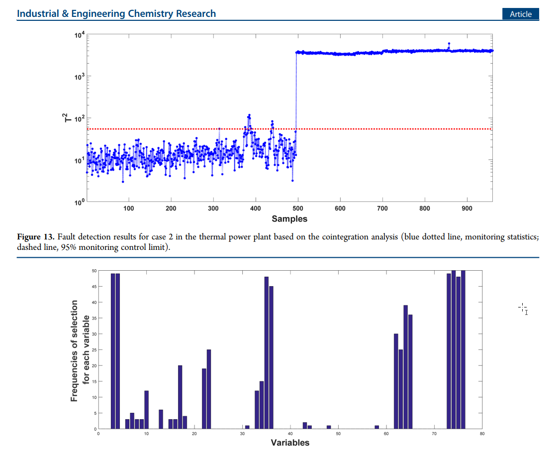
A TE process and a thermal power plant case

The thermal system of a power plant mainly includes two subsystems, steam turbine system and boiler system.

Case 1

Data

159 variables including pressure, temperature, water level, flow and so on
2880 normal samples
960 faulty samples

Process

After AFD, 51 variables are assumed to be nonstationary.
Use the 51 variables to construct a CA model, and the cointegration vectors $B (51 \times 42)$ are obtained.
Use the cointegration vectors to calculate $T^{2}$ for fault detection.
Use the sparse reconstruction method to identify the faulty variables.

Case 2

Data

154 variables
2880 normal samples to construct the cointegration model.
960 fault samples are used to online monitoring.

Process

76 variables are used after AFD test to construct the model.
Same as above

4. Fault Detection and Diagnosis Based on Sparse PCA and Two-Level Contribution Plots

#PCA #sparse-modeling #multiblock

Introduction

Fault reconstruction and contribution plot are two widely used fault diagnosis methods. But conventional contribution plot has two drawbacks:

smearing effect: in a traditional contribution plot, the contribution of a process variable consists of two parts: the individual contribution and the cross-contributions from other variables. The faulty variables can increase the contribution of fault-free variables.

the traditional contribution plot does not take into account the meaningful correlations between process variables.

The hierarchical contribution plots have been developed to improve the fault diagnosis performance. Its basic idea is to divide the overall process into seven blocks based on process knowledge, and to examine the block-wise variable contributions to identify the faulty variables responsible for the fault.

A shortcoming of the standard PCA is that its loading vectors lack sparsity; A loading vector is thus often related to most input variables. Sparse PCA aims to obtain a set of sparse loading vectors (with fewer nonzero elements) that explain most of the variance in the data.Sparse PCA has a much better interpretability than PCA, but three problems need to be solved:

how to determine the optimal sparsity (i.e., the number of nonzero elements) of each loading vector

how to choose appropriate sparse loading vectors for building a high-performance monitoring model

how to utilize the sparse characteristics
of loading vectors to improve the fault diagnosis reliability and accuracy

Methods

Sparse PCA

p = \arg max_{p} p^{t} A p

s . t . p^{T} p = 1, ∥ p ∥_{0} \leq r

where $∥ p ∥_{0}$ denotes the cardinality (the number of nonzero elements) of the vector $p$ .

Absorbing the cardinality constraint into the objective function:

p = \arg max_{p} p^{T} A p - ρ ∥ p ∥_{0}

s . t . p^{T} p = 1

Fault detection

A fault detectability matrix is defined below to construct the sparse loading matrix

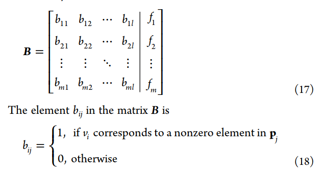
Using the $T^{2}$ and SPE statistics to detect faults.

Two-level contribution plot

The variables corresponding to nonzero elements in the same loading vector can be regarded as a variable group.

Cases

TE process

5. Fault detection and diagnosis of dynamic processes using weighted dynamic decentralized PCA approach

#PCA #Dynamic #multiblock

Introduction

Based on an argument that some process variables can inﬂuence other process variables with time-delays, a time-delayed process variable might have a stronger relationship with other variables than the non-delayed one. Therefore, there exists high correlation among process variables with time-delays.

Given that modern industrial plants are usually composed of many processing units, the resulted large-scale problem was usually at- tempted by decentralized/distributed modeling methods. Decomposing process variables into conceptually meaningful overlapping or disjoint blocks through using purely data-based methods become a popular solution to decentralized/distributed monitoring.

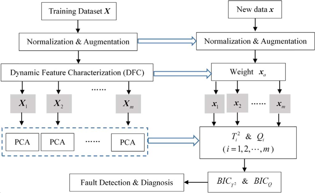
Methods

Dynamic PCA; decentralized monitoring

select dynamic feature of the process variables
split the augmented matrix $X_{a}$ into m blocks
perform PCA to each block and get $T^{2}$ and SPE for each block
Bayesian inference is employed to combine all the local results into two probabilistic monitoring indices, $B I C_{T 2}$ and $B I C_{Q}$

Cases

TE process

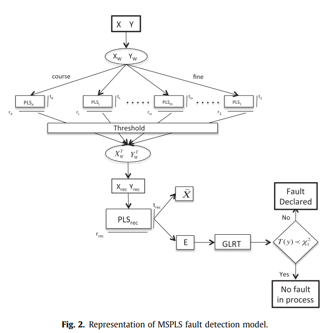
7. Multiscale PLS-based GLRT for fault detection of chemical processes

#Multiscale #PLS

Introduction

Process residuals used for the input model-based fault detection techniques may often contain high levels of noise, be highly correlated and non-Gaussian, and these may affect the fault detection performance.

Measured process data are usually contaminated with errors that mask the important features in the data and reduce the effectiveness of any fault detection method in which these data are used. Unfortunately chemical process data (as in the case of most practical data) usually possess multiscale characteristics, meaning that they contain features and noise that occur at varying contributions over time and frequency.

The kernel PLS-based generalized likelihood ratio test (GLRT) is proposed by Botre et al., and provides optimal properties by maximizing the fault detection probability for a particular false alarm rate.

Methods

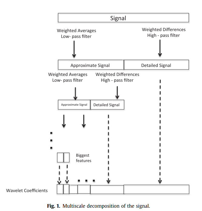
Multiscale wavelet-based data representation

Wavelet transformation is used to decompose original signal into its multiscale components characterized by time and frequency. Discrete wavelet transform (DWT) projects original signal onto orthogonal signal to obtain coarse approximate scale, the discrete wavelet function for coarse approximate scale.